Contact Us

Home

Products and Services
Software Products
Consulting
Recommended Books

Bibliography and White Papers
Free Downloads

Links

Sample Course: An Introduction to Risk Management

An introduction to Risk Management

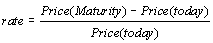
"If you can't measure it then you can't manage it," is a common saying that justifies many quantitative methods.  The following pages provide an introduction to risk assessment and risk management from a quantitative perspective, with a focus on financial applications. 

In some sense, risk is a statistical description of danger — an attribute that rational beings seek to minimize. Predicting natural, political, and financial disasters are difficult, to say the least, unless one is as pessimistic as Pascal. His point is that since disasters happen so often, then over a long time horizon, any indicator will predict one.

On the other hand, a description of risk purely in terms of mathematical expectation is misleading, since this sense of risk replaces the risk of an individual with the risk of an average. In other words, the probability that somebody wins the New York Lottery is 100%, but the likelihood that you will win the lottery is very small.  From a financial perspective, this is what can get investors into trouble.

Over the past years, we have seen how the risks associated with currency devaluation, interest rate movements, leverage in derivative markets, and "the irrational exuberance" over some equities led to near-disasters for some market participants, investors, and governments. Some of these situations could have been avoided if the dangers associated with these instruments were made more comprehensible. One of the responsibilities of risk professionals is to help make risk assessment understandable and measurable.

 Uncertainty and Risk Assessment: Background

In an uncertain world, events may not turn out the way they are supposed to. Decisions that seemed correct at one time may, on retrospect, have been wrong because of the way actual events played out. The mistake was on relying on an incorrect model of the world at the time the decision was made.

Risk assessment is concerned with understanding the effects of adverse events on a decision, plan, or value of an asset: an assessment not of what did happen in the past but of what could happen in the future. If we can understand how adverse events will change the world then we can insure (or hedge) against them by preparing for that "rainy day." This one of the goals of risk management.

From a quantitative perspective, risk assessment requires a mathematical model of the world consisting of several input factors that are related to a measurable output. A natural setting for such a model is in the realm of probability and statistics. If we assume that we know the underlying probability distribution on how events will play out — and the precise relationship of the input factors to the output results — then risk assessment is reduced to estimating the likelihood of these adverse events occurring over a given time horizon. Once the model is in place, insurance costs can be calculated.

Model Risk, Operational Risk, Compliance Risk

Unfortunately, the only way to estimate a future probability distribution is to estimate a past probability distribution (a statistical problem) and hope that the past and future distributions are not too much different (the so-called stationary assumption). This assumption is reasonable in some domains (e.g., identifying a signal from natural noise in the domain of radio communication) but not reasonable in other domains (e.g., identifying a profitable security in an emerging market). Moreover, the mathematical model may have insufficient factors, the wrong factors, or the wrong functional relationship. This induces a risk in using the model per se, called model risk.

Model risk is seen when different models react differently to different events, and produce different answers (which may or may not be correct or "good enough"). Many problems associated with model risk are due to incompleteness inherent in any model — there is no such thing as a perfect model:

• The models may be based on an incomplete theory or an inadequate theoretical approximation.
• The model inputs may be incomplete because some important factors have not been included.
• The model outputs may be incomplete because they require additional interpretation. (This is especially true for models with uncertain outcomes, like a weather forecast or an economic assessment.)

Other problems associated with model risk can be traced to the statistical methodology used to compute model parameters. This operational risk includes parameter estimation risk: the differences in results due to estimating the model parameters in different ways.

For example, suppose we want to estimate the likelihood of a hit the next time a ball player comes up to bat. How do we base our estimates on performance? Is past performance an indicator of future performance? Is aging (the player's or the bat's) a factor ? Should we calculate a batting average over the last ten games or over the last ten years? Should we take into account where the games are played and under what weather or field conditions? Should we compare the player's average to the team average? Should we just use an individual performance in computing the average, or should we include the performance of other team members as well (to create a Stein estimator)?

Note that similar problems occur when assessing performance of investments or advisors except that the warning is more explicit (as seen in the oft-repeated phrase in the advertising copy for mutual funds, "Past performance cannot guarantee future results.")

Of course, the risk in not using a quantitative model (and relying on judgement alone) exposes another aspect of model risk: these are errors in judgement are due to anchoring, inconsistency, selectivity, fallacy, and representation.

Many of these problems associated with model risk are discussed in detail in

• A Knowledge-Based Methodology for Tuning Analytical Models

Models ultimately have to be implemented as a software component or system. The act of implementing a model induces operational risk.

Different implementations of the same model may also perform differently or react differently to different adverse events, or may simply stop working at a particular moment in time. A famous example of this type of operational risk is the current "Y2K" problem associated with an implementation of the calendar: some implementations represented a year between 1900 and 1999 by the last two digits. What happened to systems that relied on these implementations in the year 2000?

What is even worse, a model or the underlying implementation may not even be testable: a testable model or implementation should be observable and controllable: it should not exhibit any test input-output inconsistencies. Here, observability refers to the ease of determining if specified inputs affect the outputs; controllability refers to the ease of producing a specified output from a specified input. A model or implementation that is not easily testable may cause several problems, as discussed in

• Testability of Software Components

On the other hand, other implementations may just simply "blow up." Thomas Edison was an eye-witness of a few operational disasters on Wall Street (including the "Black Friday" of 1869):

• Operational Risk and Real-Time Electronic Trading (1868-69)

In those days, the chemical batteries — used to generate electricity to power the telegraphs — would frequently explode. Power failures are still a concern on Wall Street.

Finally, even if all these are implemented correctly there may be legal or compliance risk due to obligations to regulatory bodies. Regulatory organizations try to guarantee safety or prevent illegal activities. For example, in the U.S., some regulatory governmental agencies include:

• Occupational Safety and Health Administration
• Department of Transportation
• Environmental Protection Agency
• Federal Trade Commission
• Securities Exchange Commission
• NASD Regulation

Not being in compliance with rules can be costly. Some activities can put a firm at risk for being fined or for being put out of business.

Financial Risk Assessment

The specific problem here is to assess the value of a security or portfolio of securities given an adverse event: an assessment of "When bad things happen to good portfolios." For example, recent sudden changes in credit and interest rates (which may or may not be due to economic, political, or emotional factors) have had devastating effects on some security prices and ultimately on the financial health of some portfolios (and some investment firms).

Some quantitative models of securities are based on factors that can be directly observed from "the market" (such as security prices, interest rates, or currency exchange rates) — at any time the security is traded or when a price is quoted. Other models are based on factors that can not be directly observed from the market (such as credit ratings, inflation indicators, or monetary indices).

Some non-market factors are made available through periodically published government or agency reports, for example, through the Federal Reserve's FRED database. Other factors, such as credit ratings, are provided by vendors (such as Standard & Poor's) or by proprietary research.

Aspects of model risk that are specific to financial models are discussed in

• Artificial Intelligence on Wall Street

Traditionally, market and non-market factors are modeled as separate components and integrated later.

Market Risk: A Simple Model of Returns

One model of security prices assumes that the security returns over a given time period are reasonably constant. A formula for the daily return on a security is

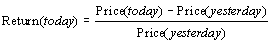
A savings bank account is an example of an riskless investment that provides a constant return. For example, if a savings account pays 3% per year, if we deposit $100 today, we will get $103 in one year (=100+3%*100).

A formula that expresses this relationship is

This relationship can also be seen in the following charts:

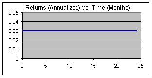
These charts graph the simple return of a security (set at a 3% annual return) and its corresponding price over the next 24 months. Note that the appealing aspect of a savings account is that returns and price are predictable by contractual commitment and that returns compound.

For example, the value in 2 years is the value after the first year plus the return on that amount after one year, or

Price(end of 2 years) = [ Price(end of 1year) ]+ 3%*[Price(end of 1 year)]

Price(end of 2 years) =[100 + 3%*100] + 3%*[100 + 3%*100] = $106.09.

This complicated expression can be factored to 100*(1+3%)*(1+3%). Note that compounding includes the return on the return.

There are other methods of reckoning returns that depend on the bank account or contractual arrangement. Returns depend on the frequency of compounding (e.g., the return can be compounded annually as above, or can be compounded quarterly, monthly, or daily, hourly, or even continuously). There are returns that depend on how one represents the number of days in a year (e.g., usually 365 days, but what if the year is a leap year? If we assume all months have 30 days then we get a 360-day year. ). The good news is that there are conversion formulas that represent one of these returns in terms of other returns — just like the formulas for converting meters to inches. When evaluating the returns of bank accounts or other contracts, we need to have to have a common return language.

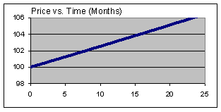
So far the model does not include risk. Returns and market prices for a risky security (like a stock) have sudden increases and decreases and look something like this:

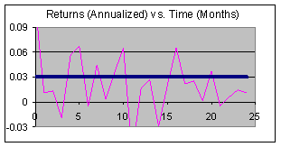
Note that the returns can even be negative (which can lead to a loss instead of a profit). Risky returns and market prices exhibit "noise." (One reason for such "noise" is that prices depend on free and open markets and these markets depend on people with conflicting goals, requirements, and emotions. All of these factors are integrated by what Adam Smith called "the invisible hand" to form a price.) These two charts superimpose the noisy return (and price) paths over the riskless paths: they show on retrospect, the returns and prices of a risky security over the last 24 months.

Can we predict future returns and prices with certainty? If we know how returns and market prices evolve then we may be able to determine likely values of returns and prices. One simple model assumes that the returns over a short time period follow the bell-shaped normal probability distribution. For example, we can assume that daily returns cluster around a mean or average: on some occasions there are good days (higher than the average daily return) and bad days (lower than the average daily return). Note that the normal bell-curve is symmetrical around its mean.

The thickness of the bell-shaped curve (a measure of the average distance from the mean) is another parameter called the standard deviation. The standard deviation is frequently used as a proxy for volatility: the impact of sudden price changes due to unusual events.

These two parameters of the normal distribution determine the likelihood of very bad days and very good days. Consequently, if we know the parameters, then we can assess the likelihood of any price path in time from an infinite number of potential price paths. 

The following chart shows several potential price paths of a security having a mean daily return of 0.0125% (which is equivalent to a monthly return of 0.25% and an annual return of 3% a year). In some ways, it shows how prices can evolve in several parallel universes:

The simple model assumes that the mean and standard deviation of daily returns are constant in a short time period: this implies that these parameters can be estimated from an historical time series of market prices or returns.

Once we have estimated these statistical parameters, we can compute a histogram of prices over a given time horizon: a frequency chart that shows a range of prices together with the percent of time that the price will be in that range. The histogram corresponds to a vertical time slice through the above chart of potential price paths.

For example, this histogram shows the potential values of a security over the next 10 days, together with the probability of the values. It looks like a normal bell-curve, symmetric around its mean value (approximately 55). The histogram shows that the value of the security will be between 53.93 and 56.61 approximately 80% of the time:

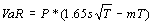
The chart also shows that the value of the security will be less 53.93 approximately 10% of the time in the next 10 days. So if the price today was actually 55, then there is a 10% chance that, in the next 10 days, we will lose 55-53.93 = 1.07 — or almost 2% (1.07/55) — of the original value of the security.

Value at Risk

Questions like

Between today and tomorrow, suppose the price moved very adversely — due to an event with a probability of occurrence of 1%. What would my loss be?"

 

What is the potential loss of a portfolio over a 5-day horizon given an adverse price movement with a 5% chance of happening?

assess what is called the Value at Risk (VaR): the VaR of a security depends on a time horizon and a probability of an adverse event occurring at the end of that horizon. Note that if the returns of the security are normally distributed, then we can derive a formula for VaR. If s denotes the (constant) daily standard deviation of the returns, and m denotes the (constant) mean return, and if the price of a security today is P, then the VaR for an adverse event with 5% probability over the next T-days is approximately

(Note that if the model assumes that the mean daily return m is zero, then we have the model and formula used by the J.P. Morgan RiskMetrics group.)

One reason for computing VaR is to establish cash reserves in case the security has to be sold at a loss. For example, the Bank of International settlement recommends that a bank should have at least three times its total 10-dayVaR (based on a 1% adverse event probability, or 2.33 standard deviations) as a cash reserve to protect itself against adverse situations.  Another reason for computing VaR is to assess how much insurance would be needed to cover potential losses.

The rationale for the multiplication factor of three is because of model risk — we observe that adverse events happen more often than predicted by a normal distribution. For most securities, the observed probability distribution of returns has "fatter tails" than a normal distribution. The factor of three effectively stretches the observed tail out to 7 standard deviations. (According to a famous result in probability theory known as Chebychev's Inequality, 7 standard deviations is actually enough to specify a 1% adverse event probability for any probability distribution symmetrical around its mean.)

A Simple Model of Portfolio Returns: Portfolio Trigonometry

For portfolios of more than one security, the standard deviation of a portfolio is not necessarily the sum of the standard deviations of the securities in the portfolio. If we still assume that the returns of the securities in the portfolio follow the simple model (all returns are normally distributed with constant standard deviation) then the return on the portfolio is a normal distribution in several dimensions — one dimension for each security — called a multivariate normal distribution. In this case, there are a set of statistical parameters that become a proxy for volatility (in addition to the individual security standard deviations), such as the covariances, and correlations.

The important effect in a portfolio is due to correlation: the statistical version of the idea "Don't put all your eggs in one basket." We can understand the effect of correlation even on a portfolio of only two securities.

Note that two securities are dependent in some time period if they consistently move in the same way (positive correlation) or if they consistently move in opposite ways (negative correlation). 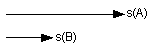For example, in a particular time period, various treasury securities are positively correlated with each other because when one treasury rises in price they all consistently rise in price; the same treasuries may be negatively correlated with stocks because over the same period when treasuries rise, stocks fall.

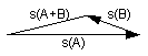
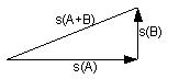
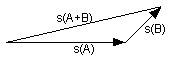
Here is an example: Astra Pharmaceuticals has symbol A, Barnes Group has symbol B. Let's construct a portfolio made up of $100 each of A and B. What is the standard deviation of the return of the portfolio?

Combining standard deviations of two securities is like combining the third side of a triangle from two given sides. For example, suppose s(A) and s(B) denote the standard deviations of the returns of A and B:

Note that in the above diagram, stock A has a larger standard deviation than stock B. It turns out that the standard deviation of the portfolio returns, denoted by s(A+B), is the magnitude of the third side of a triangle formed by s(A) and s(B).

Note that for any triangle, the sum of any two sides must be greater or equal to the third side. The missing detail that allows us to draw the triangle — the angle between s(A) and s(B) — is related to the correlation between the returns of A and B. 

Depending on the angle between them, the triangle can be either an obtuse triangle (positive correlation) —

— or an acute triangle (negative correlation) —

or a right triangle (zero correlation) —   

Computing portfolio standard deviation becomes a problem in trigonometry. For more than two securities, the correlation is measured by representing all the combinations of angles between all the individual security standard deviations.

The actual measure of positive or (negative correlation) is given by a statistical formula called the correlation coefficient: it is a number between -1 and +1 that is related to the angle between s(A) and s(B). [The correlation coefficient is actually the negative cosine of the angle between s(A) and s(B).]

So, according to portfolio trigonometry, for zero or negatively correlated securities, the standard deviation of the portfolio is always less than the sum of the standard deviations of the individual portfolio components: risk is reduced by diversifying into non-correlated asset classes. (Note that the portfolio standard deviation can even be zero if two securities have the same standard deviation and have perfect negative correlation.)

This risk management diversification technique is used extensively. One application is discussed in

• Confronting Uncertainty: Intelligent Risk Management with Futures

Of course, the big problem is assuming that correlations do not change in time (in the real world they do).

Finding the right proportional mix of securities — the one that maximize the portfolio return and minimizes the portfolio standard deviation (the proxy for risk) is a problem in optimization. If one puts additional constraints on the problem (for example, limiting the proportion of each security or prohibiting short selling) then the optimization techniques become a little involved.

Different implementation of such portfolio optimization techniques is discussed in

• A Comparison of Stochastic Search Heuristics for Portfolio Optimization

Insurance, Hedging, and Replicating Portfolios

How much does an insurance policy cost for replacing a security over a given time period? The cost of insuring an asset depends on its current price and the value of the insurance "deductible" (also known as the strike price). It also depends on the probability distribution of the value of the asset and the current interest rate.

If the returns of a security are normally distributed with zero mean, then it turns out that the 10-day VaR is equal to the cost of a 1-year zero-deductible insurance policy, guaranteeing the policy holders full replacement of the original price of the security in cash.

In the market, this insurance takes the form of a put option — a contract that protects against price losses in the security over a certain time horizon (the maturity) and below a specified price barrier (the strike price). A put option gives the holder the right to sell a security at a specified strike price at a specified time.

If the returns of a security are normally distributed with constant standard deviation, and if the current short-term interest rate is constant, a formula (the famous Black-Scholes formula) exists for pricing a put option and a call option. (A call option gives the holder the right to buy a security at a specified strike price at a specified time.)

Options can have other contractual conditions. They are an example of derivative securities — their value (an insurance cost) is derived from the value of an underlying security. In general, computing the value of a derivative security is a difficult problem in mathematical finance, especially for more complex models and contracts. For a discussion of the computational tradeoffs involved, see:

• Fast Cost-Effective Computations of Derivatives
• New Computational Architectures for Pricing Derivatives
• Assessing Alternative Technologies for the Cost-Effective Computation of Derivatives

Suppose the underlying security suffers an adverse change. What would then be the new price of an insurance policy (a put option)? A similar question is:

What is the new price of a security given a change in some underlying factor?

Suppose the price of a security depends on some underlying factor, like the interest rate. Suppose we also know how the price of the security changes when the interest rate changes. This ratio of price change to rate change is actually the slope of a line (also called the Delta) as the following figure shows:

Given an initial price and slope, we can draw a line that approximates (or predicts) the price movement based on any given interest rate movement.

We can extrapolate the line to cover any change in the underlying factor. Note that this extrapolation is only a linear approximation of what may be the actual price: the error in the approximation increases for large changes in the underlying interest rate. Conversely, the error in the approximation goes to zero as the changes in the underlying interest rate decrease to zero.

The ratio of infinitesimal price changes to infinitesimal rate changes — which approaches the slope of a tangent line at a given price — is called the first derivative. It is the instantaneous rate of change of the price with respect to the underlying factor. Note that the use of the word derivative (from differential calculus), is different from its typical use in finance relating to derivative securities.

To avoid confusion, we call the first derivative by names like Delta and Vega.

We can make a better approximation if we create another curve — by plotting different slopes over the price curve — and then look at the slope of that curve. This slope of slopes (the Delta of a Delta) is called the second derivative. To avoid confusion, we call the second derivative by names like Gamma.

Consequently, if we can compute these Deltas and Gammas then we can compute a reasonable approximation to the new price given a change in the underlying factor. Note that this result is non-parametric — it does not assume that the underlying factor or the price follows a normal distribution (or any distribution).

We can use the Black-Scholes formula for the price of an option to derive formulas for the Deltas and Gammas, relating the change in price of an option with respect to changes in its underlying. The formulas are valid as long as the returns of the underlying security are normally distributed, the returns have constant standard deviation, and the current short-term interest rate is constant.

The Deltas and Gammas are sensitivity coefficients that relate changes in underlying factors to changes in a security. They are sometimes called hedge ratios since they can be used to provide another type of insurance. Note that if two securities have the same Deltas and Gammas then they react similarly to similar changes in the underlying. So to replicate the behavior of one security (or portfolio of securities), we need to match the Deltas and Gammas in the other security (or portfolio). In general, the problem of constructing a replicating portfolio that mimics the behavior of a given security is reduced to finding the right linear combination of hedge ratios — a problem in algebra.

Credit Risk vs. Market Risk

Credit risk is concerned with to the cost of replacing an asset or contract if a party defaults on the arrangement. It could be assessed by a potential decrease in credit quality: the ability to repay obligations. Market risk is the potential loss that is associated with a market price movement. If the price movement is specified by a given probability over a specified time horizon, then, as we saw above, market risk represented as value-at-risk (VAR).

Credit quality is an attribute of a firm that is difficult to observe directly from market prices. Credit quality is assessed by different rating agencies using both a qualitative and quantitative methods. They then group credit-similar firms or parties into different credit classes or ratings. The most credit-risky class is the default class. Different agencies typically assign a "letter grade" to each class.

An example of the different factors involved in a credit quality assessment is in

•  Knowledge-Based Approaches for Evaluating Municipal Bonds

From a quantitative perspective, credit risk assessment can be measured if we can estimate or predict the probability distributions of the likelihood of default (the default probability) and the percentage of the asset that creditors can recover in the event of default (the recovery rate).

Different ratings agencies create a transition probability matrix: a table that lists the probability of going from one credit class to another over a given time period (for example, in one year). For example, the following table provides the one-year transition probabilities for a set of credit classes:

So for example:

• the probability of a A-rated firm improving its rating to an AAA in one year is 0.27%
• the probability of a A-rated firm remaining an A-rated firm is 89.05%
• the probability of a A-rated firm becoming a BBB-rated firm is 7.40%
• the probability of a A-rated firm becoming a D-rated firm (the default class) is 0.03%.

If these transition probabilities do not change from one period to the next, then a transition probability across multiple periods can be computed. (This is called the stationary Markov assumption.) Consequently, the default probability can be computed for any time period given the knowledge of the transition matrix (using a procedure called matrix multiplication). Consequently, the 2-year transition probabilities are:

Now,

• the probability of a A-rated firm improving its rating to an AAA in two years is 0.63%
• the probability of a A-rated firm remaining an A-rated firm in two years is 79.85%
• the probability of a A-rated firm becoming a BBB-rated firm in two years is 12.95%
• the probability of a A-rated firm becoming a D-rated firm (the default class) in two years is 0.10%.

Note how the transition probabilities "migrate" to lower probabilities: if we wait long enough, all risky firms will eventually have higher and higher probability of default.

Credit agencies also tabulate recovery rates for credit classes: the likely proportion of the security that a holder could recover in the case of default. Recovery rates are between 0% (recover nothing) to 100% (recover everything). All of these are statistically estimated — but not directly from market prices.

One illustration of the impact of credit risk was seen in September 1998, when the Long Term Capital investment fund was rescued by a $3.6 billion private bailout by a group of banks and brokerage firms with the coordination of the Federal Reserve. (The reason for the bailout was that Long Term Capital borrowed some of its money from its investors in the form of unsecured loans. If Long Term Capital defaulted, the investors also could have defaulted and trigger a chain reaction of further defaults.)

One trading strategy that Long Term Capital used was a credit spread: U.S. Treasury bond futures are sold short (assuming they could be bought back at a lower prices), and higher yield (and higher risk) bonds are bought with the proceeds. The strategy makes money as long as Treasury bond prices remain stable or fall. (This strategy is similar to the TED spread strategy discussed in Confronting Uncertainty: Intelligent Risk Management with Futures.) Another strategy Long Term Capital used was to invest in Russian bonds, with the assumption that United States, the International Monetary Fund and The World Bank would immediately rescue Russia from any potential default: thus rendering the default probability of Russian bonds close to zero.

The first strategy blew up when the stock market began falling in July: bond prices rose as investors chose to buy securities backed by the U.S. government (the "flight to quality and safety"). The second strategy blew up when Russia actually defaulted.

Models for Interest Rates

The simplest model for security prices assume that its returns are normally distributed in a specific time period (with constant standard deviation), and that the short-term interest rate is constant.

There are several problems with this model that are observed in practice.

First of all, none of the parameters are constant: means and standard deviation change in time. This implies that the models need to be continuously recalibrated.

A more serious problem is that interest rates are not constant. This problem is especially critical for interest rate sensitive securities such as bonds.

A bond is a security where the owner receives a fixed unconditional promise (from someone) to pay a specific principal amount of cash at a specific future date (the date when the bond matures). Unlike a stock, the price of a bond is known at some fixed future time. (The market determines the price of a bond at all other times. The market determines the price of a stock at all times — present and future.) Bonds may also pay intermediate payments (coupons or interest payments) at other times. Bonds can have other contractual conditions on the principal, interest and payment dates. For example, floating-rate bonds have variable coupons (whose value depends on an interest rate); mortgage-backed bonds have variable principal or coupons (whose value can change due to mortgage pre-payments).

Note that a bond price does not behave like a stock price: the price of a stock can range from zero to any large value (even as high as $76,600: the May 10, 1999 price of one Berkshire Hathaway class A share). A bond price is usually less than its known price at maturity: it cannot grow to any arbitrary value.

After a bond is issued, its price may fluctuate; just before it matures, its price converges to its promised payoff. This implies that the standard deviation of bond returns increases (when it is issued), fluctuates during its life, and decreases to zero at maturity. (This is known as the pull-to-par effect.)

Bond prices depend on an interest rate: the problem is which interest rate? Very simply, for a bond that does not pay any coupons (a zero-coupon bond) that matures in exactly one year, its simple annual interest rate (or "yield") is just its return:

There is an implicit interest rate for every bond issued by a government, corporation or individual. Like returns, there are formulas for interest rates that depend on the frequency of compounding (e.g., a simple interest rate compounded quarterly, monthly, annually or continuously).

There are rates that depend on how one represents the number of days in a year (e.g., the "discount" rates for 90-day U.S. treasury securities assume a 360-day year). The good news is that there are formulas that represent one of these rates in terms of other rates: we just have to agree on a common interest rate language.

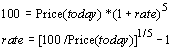
For longer time periods, the rate is its compounded return. For example, suppose the principal of a 5-year zero-coupon bond is $100. The formula linking today's price with its (annual) spot interest rate is:

This shows that the price of a bond can be given by its spot rate and vice versa. Here is another example. Suppose a 1-year treasury security promises to pay $100 in exactly one year. Today it sells for $90. Then the 1-year interest rate —called the 1-year spot rate —is then given by (100/90)-1 =11.1111% (to four decimal places).

Note that the value of $90 one year from now is

$90*(1+11.1111%) = $100.

If a 2-year treasury security promises to pay $100 in exactly two years sells for $80 today, then its 2-year spot rate is then given by

Note that because of compounding, the value of $80 two years from now is

$80*(1+11.8034%)*(1+11.8034%) = $100.

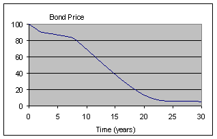
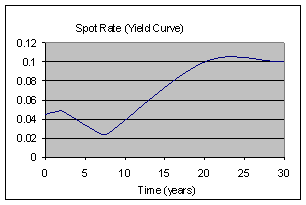
Given the appropriate bond price, we can similarly compute 2-year, 5-year, 30-year spot rates, as well as 6-month, 3-month, and 1-day spot rates.  The combination of all (zero-coupon) bond prices from an issuer create a yield curve; here is an example that shows the correspondence between yield curves of bond prices and spot interest rates:

Another interest rate is the forward rate. The forward rate is often a proxy for an unknown future spot interest rate.

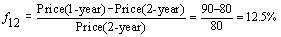
Here is an example. Suppose today is January 1, 2000, and that today's prices and rates of 1-year and 2-year zero coupon bonds are as calculated as above (the 1-year bond is $90 or 11.1111% and 2-year bond is $80 or 11.8034%). Suppose we need to borrow $100 on January 1, 2001 (in a year from now), and we will pay the money back a year after the loan is made on January 1, 2002 (which is two years from today). Given these facts, what would be the interest rate at the time of borrowing?

We really need to know the one-year spot rate on January 1, 2001. But we only know the 1-year spot rate today (which is 11.1111%); we do not know the 1-year spot rate in the future. However, we can compute an "implied" future 1-year spot rate, given the value of today's 1-year and 2-year spot rate. This 1-year forward rate from 2001 to 2002 is the rate of return from 2001 to 2002 such that, the when it is compounded with the rate from 2000 to 2001, the resultant return is the spot rate from 2000 to 2002. In other words, it is the unknown value in the following expression:

In this case the forward rate is 12.5%.

The forward rate can also be computed directly from the bond prices:

Some people believe that forward rates are predictors of future spot rates, just as they believe that forward prices of an asset or commodity are predictors of future spot prices. In general they are not. Forward rates simply correspond to the implied interest rates of bond futures: a contract that delivers a bond in a given time.

We still didn't answer the question as to what is the interest rate. The prices of all bonds issued in the U.S. are correlated to the prices of U.S. Treasuries securities: bonds backed by the credit of the U.S. government. Everyone agrees that in the U.S., these bonds are risk-free. Consequently, risk-free U.S. interest rates are determined by U.S. treasury securities. Other bonds have lower prices since they have higher risk (assuming there are no tax consequences), and their interest rates are higher (and are given by a spread over a corresponding treasury security).

Consequently, if we have a model for the U.S. risk free interest rate and a model for the credit spread, then we can theoretically price any bond in the U.S. This applies to other sovereign states as well: for example, if we have a model for the U.K. risk free interest rate and a model for the foreign exchange rate (that changes $dollars to £pounds), then we can theoretically price any U.K. bond in U.S. dollars. The trick is in developing the right interest rate model.

Historically, interest rates are rarely less than zero and never seem to grow unbounded. In ancient Babylonia, interest rates were unregulated; simple annual interest rates fluctuated between 5% to 20%. In Rome, one of the oldest interest rate regulations (450 B.C.E) fixed the interest rate to 1% per month (one thousand years later new regulations actually forbade compound interest in what remained of the Roman Empire).

In more recent times interest rates have been negative for brief periods (for example, in 1932 in the U.S. and in November 1998 in Japan).

Some interest rate models assume that spot rates do not wander from a long-term drift or mean-reverting rate. Other models are based on forward interest rates. Most are based on generalizations of the Black-Scholes model of stock returns, and are expressed in the language of stochastic differential equations.

The following Technical Note

• A Taxonomy of Interest Rate Models and Calibration Techniques

provides a brief taxonomy of some interest rate models, together with a discussion of some statistical techniques used to derive the model parameters.

Integrated Financial Risk Assessment

We introduced the section on Financial Risk Assessment with the phrase "When bad things happen to good portfolios." Here we conclude with some caveats, especially considering that "worse things can happen to a financial firm," when adverse events turn into terminal events.

Traditionally, market and non-market factors are modeled as separate components and integrated later. Market factors include those factors observable in a market, such as prices and rates. Non-market factors are not directly observable in the market, such as credit quality or compliance with regulatory procedures.

Note that some of these factors may be difficult to quantify. It may be possible to smoothly integrate a few important component risk factors. See for example, the brief Technical Note

• Models for Integrating Interest Rate, Sovereign Exchange Rate Risk, and Credit Risk

and a description of the Inductive Solutions Risk Kit system.  However, in order to integrate all component risk factors in a testable way, all factors must be observable and controllable. Otherwise, it may be difficult to decide exactly where there is a problem. Moreover, because of correlations between risks, the integration of risks may be much more than the sum of its component parts.

For example:

• Was the $1.4 billion in losses (the terminal event that forced the bankruptcy of 232-year-old Barings Bank in 1995) due to a bad futures trading model (model risk), due to settlement risk (did transfers take place as expected?), or due to lack of compliance with operating procedures?

[At the time, Barings was in the process of installing a risk management system in its Far East offices. The system was supposed to alert management to unusual company trading positions. According to Computing, (2 March 1995): "...Barings' assistant IT director, was unavailable for comment, but sources believe the bank's existing settlement system contributed to the collapse. The Cash Risk Management system was supposed to flag cash positions, but if settlements were not processed according to the bank's procedures, it could not do so. "]

• Was the terminal event that led to the 1994 collapse of Askin Capital due to interest rate risk, credit risk, model risk or due to lack of compliance with operating procedures?

[Askin Capital invested in mortgage-backed securities — bonds based on home mortgages that have a low default risk (since the payments are guaranteed by various federal government agencies). However, these bonds have prepayment risk: early repayment of mortgage principal induces an opportunity cost for the investor who is on the receiving end of the mortgage cash flows. The fund blew up in 1994, after the Federal Reserve unexpectedly raised interest rates — for the first time in five years. This sudden increase reduced the number of homeowners seeking to refinance their mortgages with new loans. This was completely counter to the prepayment assumptions made: the value of certain mortgage derivatives fell. In March 1996, the investors sued three Wall Street brokerage firms and Askin Capital Management for $700 million.]

Sometimes a firm can we doing very well financially, but may still be at risk of substantial losses. Some activities can put a firm at risk for being fined or put out of business: not being in compliance with rules can be costly. Who sets the rules? In the U.S., the Securities Exchange Commission is the U.S. agency that monitors the U.S. exchanges and markets to make sure that they are fair and orderly and in compliance with the law. Some examples of high-compliance-risk activities that the SEC monitors are listed in the

• Market Surveillance Glossary

How these high-risk activities play out (usually not for the benefit of the firm) and how compliance systems can be designed to detect them is discussed in

• Market Analysis for Risk Management and Regulation.

For example,

• In 1989, the terminal event for Drexel Burnham was their agreement to a $300 million fine to the Justice Department and to establish a $350 million fund for civil suits, resulting from their inability to properly monitor the effectiveness of their insider trading compliance procedures.
• In 1998, a federal judge approved a record $1.03 billion settlement of a class-action lawsuit by investors who accused 37 brokerages of overcharging them for Nasdaq-listed stocks in a price-rigging conspiracy. As part of this settlement, the firms also agreed to improve and monitor their best execution obligations, as discussed in the Technical Note
  • Compliance Risk and Best Execution

In these two cases, the firms were at risk due to their lack of compliance with SEC rules and regulations. An integrated financial risk assessment must take into consideration as many risk factors as possible as well as the established rules and procedures of regulatory organizations. Many of these are listed at

• Risk Watch

Risk Watch was set up by the International Finance and Commodities Institute (IFCI) — a non-profit foundation created in 1984 on the initiative of the Swiss Futures & Options Association, with the objective of promoting global understanding of commodity trading as well as financial futures and options. Risk Watch provides an introduction, glossary, and guide to the most important official documents in the area of financial risk management.

• The Global Association of Risk Professionals (GARP)

GARP is a not-for-profit, independent organization of financial risk management practitioners and researchers. GARP's mission is to serve its members by facilitating the exchange of information, developing educational programs, and promoting standards in the area of financial risk management

Many risk factors listed above are difficult to quantify and observe. On the other hand, even if we have models of these risk factors, a model that integrates them would also carry its own share of model risk.